Tutorial
This tutorial is split in three parts.
Part I treats the Genomic Dataset that are available through Janggu which can be directly consumed by your keras model. The tutorial illustates how to access genomics data from various widely used file formats, including FASTA, BAM, BIGWIG, BED and GFF for the purpose of using them as input to a deep learning application. It illustrates a range of parameters to adapt the read out of genomics data and it shows how the predictions or feature activities of a neural network in numpy format can be converted to a genomic coverage representation that can in turn be exported to BIGWIG file format or visualized directly via a genome browser-like plot.
Part II treats utilities for defining a neural networks based on keras.
Part III illustrates Janggu’s evaluation utilities.
Complementary to this tutorial, the janggu repository contains a number of jupyter notebooks that illustrate for example with keras or sklearn:
Furthermore, use cases for predicting JunD binding, training and adapting published genomics models as well as a regression model example are demonstrated in the supplementary repository: Janggu use cases
Part I) Introduction to Genomic Datasets
janggu.data provides Dataset classes
that can be used for
training and evaluating neural networks.
Of particular importance are the Genomics-specific dataset,
Bioseq and Cover which
allow easy access to genomics data,
including DNA sequences or coverage information.
Apart from accessing raw genomics data, Janggu
also facilitates a method for converting an ordinary
numpy array (e.g. predictions obtained from a neural net)
to a Cover object. This enables the user to export the predictions
as BIGWIG format or interactively plot genome browser tracks.
In this tutorial, we demonstrate some of the key functionality of
Janggu. Further details are available in Genomic Datasets
and API.
Bioseq
The Bioseq can be used to load nucleotide
or protein sequence data from
fasta files or from a reference genome
along with a set of genomic coordinates defining the region of interest (ROI).
The class facilitates access the
one-hot encoding representation of the sequences.
Specifically,
the one-hot encoding is represented as a
4D array with dimensions corresponding
to (region, region_length, 1, alphabet_size).
The Bioseq offers a number of features:
- Strand-specific sequence extraction (if DNA sequences are extracted from the reference genome)
- Higher-order one-hot encoding, e.g. di-nucleotide based
Sequences can be loaded in two ways: using
Bioseq.create_from_seq or
Bioseq.create_from_refgenome.
The former constructor method can be used to load
DNA or protein sequences from fasta files directly
or from as list of Bio.SeqRecord.SeqRecord entries.
An example is shown below:
from pkg_resources import resource_filename
from janggu.data import Bioseq

fasta_file = resource_filename('janggu',
                               'resources/sample.fa')

dna = Bioseq.create_from_seq(name='dna',
                             fastafile=fasta_file)

# there are 3897 sequences in the in sample.fa
len(dna)

# Each sequence is 200 bp of length
dna.shape  # is (3897, 200, 1, 4)

# One-hot encoding for the first 10 bases of the first region
dna[0][0, :10, 0, :]

#array([[0, 1, 0, 0],
#       [1, 0, 0, 0],
#       [0, 1, 0, 0],
#       [1, 0, 0, 0],
#       [0, 0, 1, 0],
#       [0, 1, 0, 0],
#       [1, 0, 0, 0],
#       [0, 0, 1, 0],
#       [1, 0, 0, 0],
#       [0, 0, 1, 0]], dtype=int8)
Furthermore, it is possible to trim variable sequence length using
the fixedlen option. If specfied, all sequences will be truncated
or zero-padded to length fixedlen. For example,
dna = Bioseq.create_from_seq(name='dna',
                             fastafile=fasta_file,
                             fixedlen=205)

# Each sequence is 205 bp of length
dna.shape  # is (3897, 205, 1, 4)

# the last 5 position were zero padded
dna[0][0, -6:, 0, :]

#array([[1, 0, 0, 0],
#       [0, 0, 0, 0],
#       [0, 0, 0, 0],
#       [0, 0, 0, 0],
#       [0, 0, 0, 0],
#       [0, 0, 0, 0]], dtype=int8)
Alternatively, nucleotide sequences can be obtained from a reference genome directly along with a BED or GFF file that indicates the region of interest (ROI).
If each interval in the BED-file already corresponds to a ‘datapoint’ that shall be consumed during training, like it is the case for ‘sample_equalsize.bed’, the associated DNA sequences can be loaded according to
roi = resource_filename('janggu',
                        'resources/sample_equalsize.bed')
refgenome = resource_filename('janggu',
                              'resources/sample_genome.fa')

dna = Bioseq.create_from_refgenome(name='dna',
                                   refgenome=refgenome,
                                   roi=roi)

dna.shape  # is (4, 200, 1, 4)
# One-hot encoding of the first 10 nucleotides in region 0
dna[0][0, :10, 0, :]

#array([[0, 1, 0, 0],
#       [1, 0, 0, 0],
#       [0, 1, 0, 0],
#       [1, 0, 0, 0],
#       [0, 0, 1, 0],
#       [0, 1, 0, 0],
#       [1, 0, 0, 0],
#       [0, 0, 1, 0],
#       [1, 0, 0, 0],
#       [0, 0, 1, 0]], dtype=int8)
Sometimes it is more convenient to provide the ROI
as a set of variable-sized broad intervals
(e.g. chr1:10000-50000 and chr3:4000-8000)
which should be divided into sub-intervals
of equal length (e.g. of length 200 bp).
This can be achieved
by explicitly specifying a desired binsize
and stepsize as shown below:
roi = resource_filename('janggu',
                        'resources/sample.bed')

# loading non-overlapping intervals
dna = Bioseq.create_from_refgenome(name='dna',
                                   refgenome=refgenome,
                                   roi=roi,
                                   binsize=200,
                                   stepsize=200)

dna.shape  # is (100, 200, 1, 4)

# loading mutually overlapping intervals
dna = Bioseq.create_from_refgenome(name='dna',
                                   refgenome=refgenome,
                                   roi=roi,
                                   binsize=200,
                                   stepsize=50)

dna.shape  # is (394, 200, 1, 4)
The argument flank can be used to extend
the intervals up and downstream by a given length
dna = Bioseq.create_from_refgenome(name='dna',
                                   refgenome=refgenome,
                                   roi=roi,
                                   binsize=200,
                                   stepsize=200,
                                   flank=100)

dna.shape  # is (100, 400, 1, 4)
Finally, sequences can be represented using higher-order
one-hot representation using the order argument. An example
of a di-nucleotide-based one-hot representation is shown below
dna = Bioseq.create_from_refgenome(name='dna',
                                   refgenome=refgenome,
                                   roi=roi,
                                   binsize=200,
                                   stepsize=200,
                                   order=2)

# is (100, 199, 1, 16)
# that is the last dimension represents di-nucleotides
dna.shape

dna.conditions
# ['AA', 'AC', 'AG', 'AT', 'CA', 'CC', 'CG', 'CT', 'GA', 'GC', 'GG', 'GT', 'TA', 'TC', 'TG', 'TT']

dna[0][0, :5, 0, :]

#array([[0, 0, 0, 1, 0, 0, 0, 0, 0, 0, 0, 0, 0, 0, 0, 0],
#       [0, 0, 0, 0, 0, 0, 0, 0, 0, 0, 0, 0, 0, 0, 0, 1],
#       [0, 0, 0, 0, 0, 0, 0, 0, 0, 0, 0, 0, 0, 0, 1, 0],
#       [0, 0, 0, 0, 0, 0, 0, 0, 0, 0, 0, 1, 0, 0, 0, 0],
#       [0, 0, 0, 0, 0, 0, 0, 0, 0, 0, 0, 0, 0, 0, 1, 0]], dtype=int8)
Cover
Cover can be utilized to fetch different kinds of
coverage data from commonly used data formats,
including BAM, BIGWIG, BED and GFF.
Coverage data is stored as a 4D array with dimensions corresponding
to (region, region_length, strand, condition).
The following examples illustrate some use cases for Cover,
including loading, normalizing coverage data.
Additional features are described in the API.
Loading read count coverage from BAM files is supported for single-end and paired-end alignments. For the single-end case reads are counted on the 5’-end and and for paired-end alignments, reads are optionally counted at the mid-points or 5’ ends of the first mate. The following example illustrate how to extract base-pair resolution coverage with and without strandedness.
from janggu.data import Cover

bam_file = resource_filename('janggu',
                             'resources/sample.bam')

roi = resource_filename('janggu',
                        'resources/sample.bed')

cover = Cover.create_from_bam('read_count_coverage',
                              bamfiles=bam_file,
                              binsize=200,
                              stepsize=200,
                              roi=roi)

cover.shape  # is (100, 200, 2, 1)
cover[0]  # coverage of the first region

# Coverage regardless of read strandedness
# sums reads from both strand.
cover = Cover.create_from_bam('read_coverage',
                              bamfiles=bam_file,
                              binsize=200,
                              stepsize=200,
                              stranded=False,
                              roi=roi)

cover.shape  # is (100, 200, 1, 1)
Sometimes it is desirable to determine the read
count coverage in say 50 bp bins which can be
controlled by the resolution argument.
Consequently, note that the second dimension amounts
to length 4 using binsize=200 and resolution=50 in the following example
# example with resolution=200 bp
cover = Cover.create_from_bam('read_coverage',
                              bamfiles=bam_file,
                              binsize=200,
                              resolution=50,
                              roi=roi)

cover.shape  # is (100, 4, 2, 1)
It might be desired to aggregate reads across entire interval
rather than binning the genome to equally sized bins of
length resolution. An example application for this would
be to count reads per possibly variable-size regions (e.g. genes).
This can be achived by resolution=None which results
in the second dimension being collapsed to a length of one.
# example with resolution=None
cover = Cover.create_from_bam('read_coverage',
                              bamfiles=bam_file,
                              binsize=200,
                              resolution=None,
                              roi=roi)

cover.shape  # is (100, 1, 2, 1)
Similarly, if strandedness is not relevant we may use
# example with resolution=None without strandedness
cover = Cover.create_from_bam('read_coverage',
                              bamfiles=bam_file,
                              binsize=200,
                              resolution=None,
                              stranded=False,
                              roi=roi)

cover.shape  # is (100, 1, 1, 1)
Finally, it is possible to normalize the coverage profile, e.g.
to account for differences in sequencing depth across experiments
using the normalizer argument
# example with resolution=None without strandedness
cover = Cover.create_from_bam('read_coverage',
                              bamfiles=bam_file,
                              binsize=200,
                              resolution=None,
                              stranded=False,
                              normalizer='tpm',
                              roi=roi)

cover.shape  # is (100, 1, 1, 1)
More details on alternative normalization options are discussed in Genomic Datasets.
Loading signal coverage from BIGWIG files can be achieved analogously:
roi = resource_filename('janggu',
                        'resources/sample.bed')
bw_file = resource_filename('janggu',
                            'resources/sample.bw')

cover = Cover.create_from_bigwig('bigwig_coverage',
                                 bigwigfiles=bw_file,
                                 roi=roi,
                                 binsize=200,
                                 stepsize=200)

cover.shape  # is (100, 200, 1, 1)
When applying signal aggregation using e.g resolution=50 or resolution=None,
additionally, the aggregation method can be specified using
the collapser argument.
For example, in order to represent the resolution sized
bin by its mean signal the following snippet may be used:
cover = Cover.create_from_bigwig('bigwig_coverage',
                                 bigwigfiles=bw_file,
                                 roi=roi,
                                 binsize=200,
                                 resolution=None,
                                 collapser='mean')

cover.shape  # is (100, 1, 1, 1)
More details on alternative collapse options are discussed in Genomic Datasets.
Coverage from a BED files is largely analogous to extracting coverage
information from BAM or BIGWIG files, but in addition the mode option
enables to interpret BED-like files in various ways:
mode='binary'Presence/Absence mode interprets the ROI as the union of positive and negative cases in a binary classification setting and regions contained inbedfilesas positive examples.mode='score'reads out the real-valued score field value from the associated regions.mode='score_category'transforms integer-valued scores into a categorical one-hot representation.mode='name_category'transforms the name field into a categorical one-hot representation.mode='bedgraph'reads in the score from a file in bedgraph format.
Examples of loading data from a BED file are shown below
roi = resource_filename('janggu',
                        'resources/sample.bed')
score_file = resource_filename('janggu',
                               'resources/scored_sample.bed')

# binary mode (default)
cover = Cover.create_from_bed('binary_coverage',
                              bedfiles=score_file,
                              roi=roi,
                              binsize=200,
                              stepsize=200,
                              collapser='max',
                              resolution=None)

cover.shape
# (100, 1, 1, 1)

cover[4]
# array([[[[1.]]]])

# score mode
cover = Cover.create_from_bed('score_coverage',
                              bedfiles=score_file,
                              roi=roi,
                              binsize=200,
                              stepsize=200,
                              resolution=None,
                              collapser='max',
                              mode='score')

cover.shape
# (100, 1, 1, 1)

cover[4]
# array([[[[5.]]]])


# scoreclass (or categorical) mode
# Interprets the integer-valued score as class-label,
# which will then be one-hot encoded.
cover = Cover.create_from_bed('cat_coverage',
                              bedfiles=score_file,
                              roi=roi,
                              binsize=200,
                              stepsize=200,
                              resolution=None,
                              collapser='max',
                              mode='score_category')

# there are 4 categories
cover.shape
# (100, 1, 1, 4)

# category names
cover.conditions
# ['1', '2', '4', '5']

cover[4]
# array([[[[0., 0., 0., 1.]]]])

# nameclass mode
# Interprets the name field as class-label.
# The class labels will be one hot encoded.
cover = Cover.create_from_bed('cat_coverage',
                              bedfiles=score_file,
                              roi=roi,
                              binsize=200,
                              stepsize=200,
                              resolution=None,
                              collapser='max',
                              mode='name_category')

cover.shape
# (100, 1, 1, 2)

# category names
cover.conditions
# ['state1', 'state2']

cover[4]
# array([[[[0., 1.]]]])

# bedgraph-format mode
bedgraph_file = resource_filename('janggu',
                                  'resources/sample.bedgraph')

cover = Cover.create_from_bed('bedgraph_coverage',
                              bedfiles=bedgraph_file,
                              roi=roi,
                              binsize=200,
                              stepsize=200,
                              resolution=None,
                              collapser='max',
                              mode='bedgraph')

cover.shape
# (100, 1, 1, 1)

cover[4]
# array([[[[0.5]]]])
Dataset wrappers
In addition to the core datset Bioseq and Cover, Janggu offers convenience wrappers
to transform them in various ways.
For instance, ReduceDim can be used to convert a 4D coverage dataset into 2D table like object.
That is it may be used to transform the dimensions
(region, region_length, strand, condition) to (region, condition) by
aggregating over the middle two dimensions.
from janggu.data import ReduceDim

cover.shape
# (100, 1, 1, 1)

data = ReduceDim(cover, aggregator='sum')

data.shape
# (100, 1)
Other dataset wrappers can be used in order to perform data augmentation, including
RandomSignalScale and RandomOrientation which can be used
to randomly alter the signal intensity during model fitting and randomly flipping
the 5’ to 3’ orientations of the coverage signal.
For more specialized cases, these wrappers might also be a good starting point to derive or adapt from.
Using the Genomic Datasets with keras or sklearn
The above mentioned datasets Bioseq and Cover
are directly compatible with keras and sklearn models. An illustration of a
simple convolutional neural network with keras is shown in
keras cnn example.
Moreover, an example of a logistic regression model from sklearn used with Janggu
is shown in
sklearn example.
Converting a Numpy array to Cover
After having trained and performed predictions with a model, the data
is represented as numpy array. A convenient way to reassociate the
predictions with the genomic coordinates they correspond to is achieved
using create_from_array.
import numpy as np

# True labels may be obtained from a BED file
cover = Cover.create_from_bigwig('cov',
                                  bigwigfiles=bw_file,
                                  roi=roi,
                                  binsize=200,
                                  resolution=50)


# Let's pretend to have derived predictions from a NN
# of the same shape
predictions = np.random.randn(*cover.shape)*.1 + cover[:]

# We can reassociate the predictions with the genomic coordinates
# of a :code:`GenomicIndexer` (in this case, cover.gindexer).
predictions = Cover.create_from_array('predictions',
                                      predictions, cover.gindexer)
Exporting and visualizing Cover
After having converted the predictions or feature activities of a neural
network to a Cover object, it is possible to export the results
as BIGWIG format for further investigation in a genome browser of your choice
# writes the predictions to a specified folder
predictions.export_to_bigwig(output_dir = './')
which should result in a file ‘predictions.Cond_0.bigwig’.
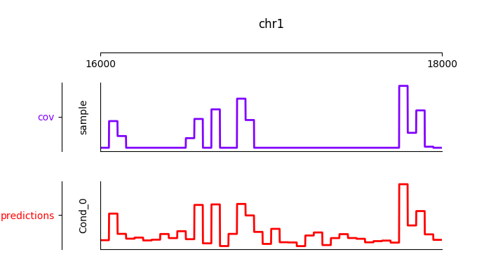
Furthermore, it is possible to visualize the tracks interactively
from janggu.data import LineTrack
from janggu.data import plotGenomeTrack

fig = plotGenomeTrack([LineTrack(cover), LineTrack(predictions)], 'chr1', 16000, 18000).figsave('coverage.png')
Part II) Building a neural network with Janggu
While the Genomic Dataset may be used directly with keras,
this part of the tutorial discusses the Janggu wrapper class
for a keras model.
It offers the following features:
- Building models using automatic input and output layer shape inference
- Built-in logging functionality
- Automatic evaluation through the attachment of Scorer callbacks
A list of examples can be found in the Table at the beginning.
A neural network can be created by
instantiating a Janggu object.
There are two ways of achieving this:
- Similar as with keras.models.Model, a
Jangguobject can be created from a set of native keras Input and Output layers, respectively. - Janggu offers a Janggu.create constructor method which helps to reduce redundant code when defining many rather similar models.
Example 1: Instantiate Janggu similar to keras.models.Model
from keras.layers import Input
from keras.layers import Dense

from janggu import Janggu

# Define neural network layers using keras
in_ = Input(shape=(10,), name='ip')
layer = Dense(3)(in_)
output = Dense(1, activation='sigmoid',
               name='out')(layer)

# Instantiate model name.
model = Janggu(inputs=in_, outputs=output)
model.summary()
Example 2: Specify a model using a model template function
As an alternative to the above stated variant, it is also possible to specify a network via a python function as in the following example
def model_template(inputs, inp, oup, params):
    inputs = Input(shape=(10,), name='ip')
    layer = Dense(params)(inputs)
    output = Dense(1, activation='sigmoid',
                   name='out')(layer)
    return inputs, output

# Defines the same model by invoking the definition function
# and the create constructor.
model = Janggu.create(template=model_template,
                      modelparams=3)
The model template function must adhere to the
signature template(inputs, inp, oup, params).
Notice, that modelparams=3 gets passed on to params
upon model creation. This allows to parametrize the network
and reduces code redundancy.
From the model template it is also possible to obtain a keras model directly, rather than the Janggu model wrapper if this is preferred
from janggu import create_model

# This will construct a keras model directly
model = create_model(template=model_template,
                     modelparams=3)
Example 3: Automatic Input and Output layer extension
A second benefit to invoke Janggu.create is that it can automatically
determine and append appropriate Input and Output layers to the network.
This means, only the network body remains to be defined.
import numpy as np
from janggu import inputlayer, outputdense
from janggu.data import Array

# Some random data
DATA = Array('ip', np.random.random((1000, 10)))
LABELS = Array('out', np.random.randint(2, size=(1000, 1)))

# inputlayer and outputdense automatically
# extract dataset shapes and extend the
# Input and Output layers appropriately.
# That is, only the model body needs to be specified.
@inputlayer
@outputdense('sigmoid')
def model_body_template(inputs, inp, oup, params):
    with inputs.use('ip') as layer:
        # the with block allows
        # for easy access of a specific named input.
        output = Dense(params)(layer)
    return inputs, output

# create the model.
model = Janggu.create(template=model_body_template,
                      modelparams=3,
                      inputs=DATA, outputs=LABELS)
model.summary()
As is illustrated by the example, automatic Input and Output layer determination
can be achieved by using the decorators inputlayer and/or
outputdense which extract the layer dimensions from the
provided input and output Datasets in the create constructor.
Fit a neural network on DNA sequences
In the previous sections, we learned how to acquire data and how to instantiate neural networks. Now let’s create and fit a simple convolutional neural network that learns to discriminate between two classes of sequences. In the following example the sample sequences are of length 200 bp each. sample.fa contains Oct4 CHip-seq peaks and sample2.fa contains Mafk CHip-seq peaks. We shall use a simple convolutional neural network with 30 filters of length 21 bp to learn the sequence features that discriminate the two sets of sequences.
The example makes use of two more janggu utilities: First,
DnaConv2D constitutes a keras layer wrapper that facilitates scanning
of both DNA strands with the same kernels. That is it simulataneously applies
a convolution and a cross-correlation and aggregates the resulting activities.
Second, the example illustrates the dataset wrapper ReduceDim which
allows to collapse 4D the signal contained in the Cover object
across the sequence length and strand dimension. The result is yields a 2D
table-like dataset which is used in the subsequent model fitting example.
from keras.layers import Conv2D
from keras.layers import GlobalAveragePooling2D
from janggu import inputlayer
from janggu import outputconv
from janggu import DnaConv2D
from janggu.data import ReduceDim


# load the dataset which consists of
# 1) a reference genome
REFGENOME = resource_filename('janggu', 'resources/pseudo_genome.fa')
# 2) ROI contains regions spanning positive and negative examples
ROI_FILE = resource_filename('janggu', 'resources/roi_train.bed')
# 3) PEAK_FILE only contains positive examples
PEAK_FILE = resource_filename('janggu', 'resources/scores.bed')

# DNA sequences are loaded directly from the reference genome
DNA = Bioseq.create_from_refgenome('dna', refgenome=REFGENOME,
                                   roi=ROI_FILE,
                                   binsize=200)

# Classification labels over the same regions are loaded
# into the Coverage dataset.
# It is important that both DNA and LABELS load with the same
# binsize, stepsize to ensure
# the correct correspondence between both datasets.
# Finally, the ReduceDim dataset wrapper transforms the 4D Coverage
# object into a 2D table like object (regions by conditions)
LABELS = ReduceDim(Cover.create_from_bed('peaks', roi=ROI_FILE,
                               bedfiles=PEAK_FILE,
                               binsize=200,
                               resolution=None), aggregator='mean')


# 2. define a simple conv net with 30 filters of length 15 bp
# and relu activation.
# outputconv as opposed to outputdense will put a conv layer as output
@inputlayer
@outputdense('sigmoid')
def double_stranded_model(inputs, inp, oup, params):
    with inputs.use('dna') as layer:
        # The DnaConv2D wrapper can be used with Conv2D
        # to scan both DNA strands with the weight matrices.
        layer = DnaConv2D(Conv2D(params[0], (params[1], 1),
                                 activation=params[2]))(layer)

    output = GlobalAveragePooling2D(name='motif')(layer)
    return inputs, output


# 3. instantiate and compile the model
model = Janggu.create(template=double_stranded_model,
                      modelparams=(30, 15, 'relu'),
                      inputs=DNA, outputs=LABELS)
model.compile(optimizer='adadelta', loss='binary_crossentropy',
              metrics=['acc'])

# 4. fit the model
model.fit(DNA,LABELS,epochs=100)
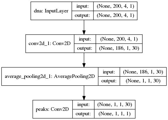
An illustration of the network architecture is depicted below.
Upon creation of the model a network depiction is
automatically produced in <results_root>/models which is illustrated
below
After the model has been trained, the model parameters and the
illustration of the architecture are stored in <results_root>/models.
Furthermore, information about the model fitting, model and dataset dimensions
are written to <results_root>/logs.
Note that in the example above the output dimensionality of the network is 4D.
However, it might be more convenient at times to remove the single dimensional
elements of the array.
This can be achieved by wrapping the LABELS dataset using ReduceDim.
In this case the example becomes
@inputlayer
@outputdense('sigmoid')
def double_stranded_model(inputs, inp, oup, params):
    with inputs.use('dna') as layer:
        # The DnaConv2D wrapper can be used with Conv2D
        # to scan both DNA strands with the weight matrices.
        layer = DnaConv2D(Conv2D(params[0], (params[1], 1),
                                 activation=params[2]))(layer)

    output = GlobalAveragePooling2D(name='motif')(layer)
    return inputs, output


# 3. instantiate and compile the model
model = Janggu.create(template=double_stranded_model,
                      modelparams=(30, 15, 'relu'),
                      inputs=DNA, outputs=LABELS)
model.compile(optimizer='adadelta', loss='binary_crossentropy',
              metrics=['acc'])

# 4. fit the model
model.fit(DNA, LABELS, epochs=100)
Part III) Evaluation and interpretation of the model
Janggu supports various methods to evaluate and interprete a trained model, including evaluating summary scores, inspecting the results in the built-in genome browser (see Part I), evaluating the integrated gradients which allows to visualized input feature importance and by offering support for variant effect predictions. In this last part we will illustrate these aspects.
Evaluation of summary scores
After the model has been trained, the quality of the predictions is usually summarized by its agreement with the ground truth, e.g. by evaluating the area under the ROC curve in a binary classification application or by computing the correlation between predictions and targets in a regression setting.
For some commonly used evaluation criteria, the evaluate method directly allows to determine and export the given metric results. For example, for a classification task the following line evaluates the ROC and PRC and exports a figure and a tsv file, respectively, for each measure.
model.evaluate(DNA_TEST, LABELS_TEST, callbacks=['roc', 'prc', 'auprc', 'auroc'])
The results are stored in <results_root>/evaluation/{roc,prc}.png
as well as <results_root>/evaluation/{auroc,auprc}.tsv.
Furthermore, for a regression setting it is possible to invoke
model.evaluate(DNA_TEST, LABELS_TEST, callbacks=['cor', 'mae', 'mse', 'var_explained'])
which evaluates the Pearson’s correlation, the mean absolute error, the mean squared error and the explained variance into tsv files.
It is also possible to customize the scoring callbacks by instantiating a
Scorer objects which can be passed to
model.evaluate and model.predict. Further details about
customizing the scoring callbacks are given in Customize Evaluation.
Input feature importance
In order to inspect what the model has learned, it is possible to identify the most important features in the input space using the integrated gradients method.
This is illustrated on a toy example for discriminating Oct4 and Mafk binding sites (see variant effect prediction).
Variant effect prediction
In order to measure the effect of single nucleotide variant on the predict
network output can be tested via the Janggu.predict_variant_effect
based on a Bioseq object and single nucleotide variants in VCF format.
This method evaluates the network for each variant (using its sequence context)
as well as its respective reference sequence.
As a result, an hdf5 file and a bed file will be produced which
contain the network predictions for each variant and the associated genomic
loci.
An illustration of the variant effect prediction in the notebook (see
variant effect prediction).
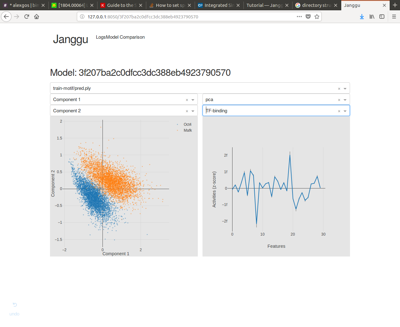
Browse through the results
Finally, after you have fitted and evaluated your results you can browse through the results in an web browser of your choice.
To this end, first start the web application server
janggu -path <results-root>
Then you can inspect the outputs in a browser of your choice (default: localhost:8050)